Advanced Machine Learning Approaches for Detecting Trolls on Twitter

Content Warning

This report includes texts written by internet trolls, many of which are extremely offensive.

Abstract

Social media platforms such as Twitter have revolutionized how people interact, share information, and express their opinions. However, this rapid expansion has also brought with it an alarming rise in malicious activities, with online trolls exploiting the platform to spread hate, misinformation, and toxicity. Detecting and mitigating such trolls have become critical in maintaining a healthy digital environment and safeguarding the well-being of users.

In this report, I present an exploratory investigation into the development of a cutting-edge machine learning model for the identification and classification of trolls on Twitter. In particular, I train and test three model architectures: Partial least squares (PLS) regression, boosting, and a fine-tuned transformer neural network.

Exploratory Analysis and Feature Selection

The training data for this report consist of short texts from Twitter, each manually labeled with label indicating whether it is or is not a troll.

library(tidyverse)

── Attaching core tidyverse packages ──────────────────────── tidyverse 2.0.0 ──
✔ dplyr     1.1.4     ✔ readr     2.1.4
✔ forcats   1.0.0     ✔ stringr   1.5.1
✔ ggplot2   3.4.4     ✔ tibble    3.2.1
✔ lubridate 1.9.3     ✔ tidyr     1.3.0
✔ purrr     1.0.2     
── Conflicts ────────────────────────────────────────── tidyverse_conflicts() ──
✖ dplyr::filter() masks stats::filter()
✖ dplyr::lag()    masks stats::lag()
ℹ Use the conflicted package (<http://conflicted.r-lib.org/>) to force all conflicts to become errors

library(wordcloud)

Loading required package: RColorBrewer

library(tidytext)
library(caret)

Loading required package: lattice

Attaching package: 'caret'

The following object is masked from 'package:purrr':

    lift

library(pls)

Attaching package: 'pls'

The following object is masked from 'package:caret':

    R2

The following object is masked from 'package:stats':

    loadings

library(varrank)

load("troll_classification.RData")

# train <- read_csv("train.csv") %>% mutate(label = factor(label))
# test <- read_csv("test.csv")

head(train)

# A tibble: 6 × 3
  rowid content                                                            label
  <dbl> <chr>                                                              <fct>
1     1 'How to Talk to Girls'. I'm going to write a gay centred spinoff … 0    
2     2 'Turns out not where but who you're with that really matters.' ;)… 0    
3     3 'you can do it!' kick ass fdo!                                     0    
4     4 --- each confit will make the fat saltier (it's already pretty sa… 0    
5     5 --- that shit right there fool ... is FUCKING TIGHT!!!! --- http:… 1    
6     6 --- you may be working from the same book as me; I'm confiting po… 0    

These data represent a more difficult classification task than many real-world applications, as no information is given about thread-level context or other texts produced by the same account. This report will focus purely on features of the individual text.

Word Clouds

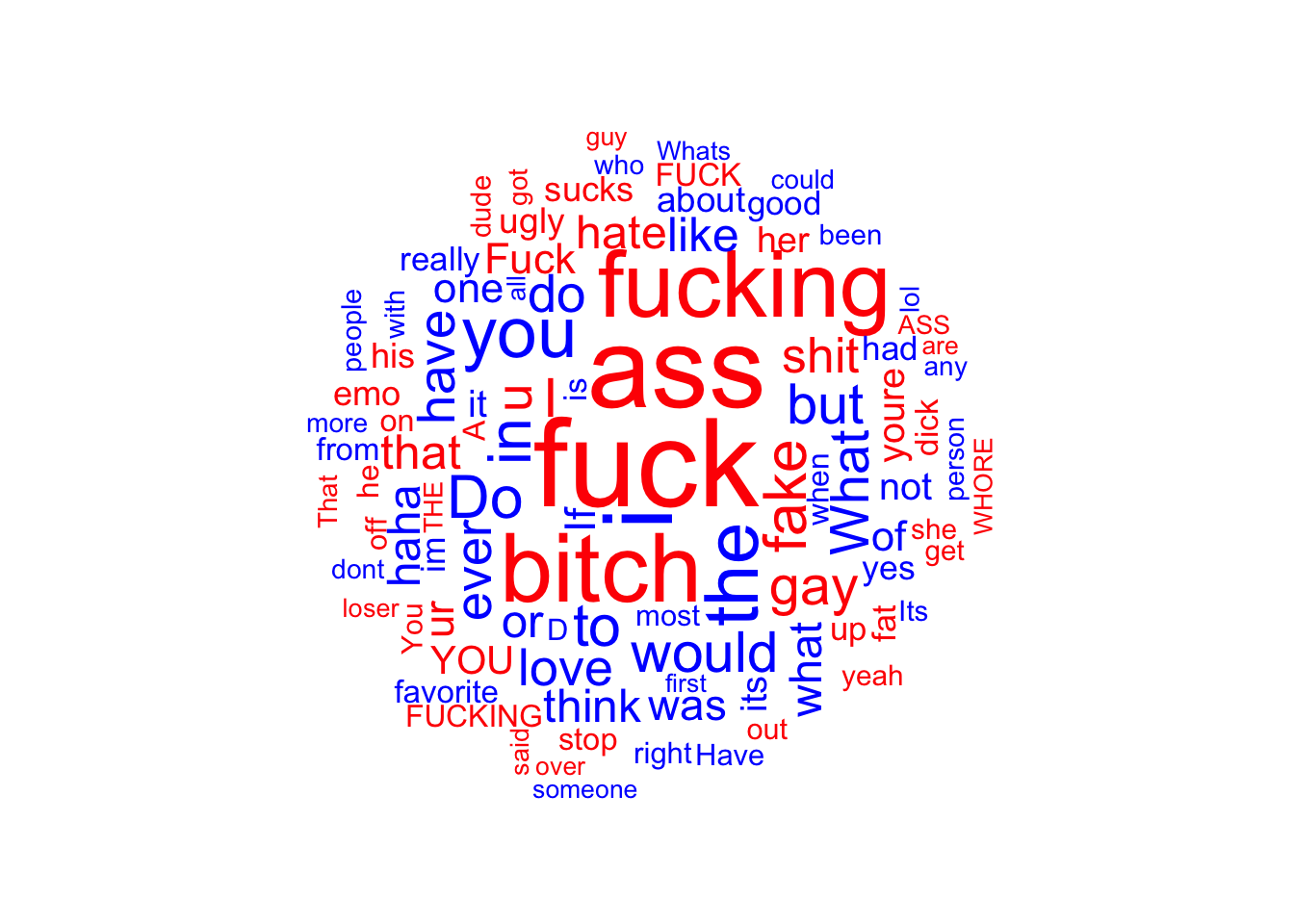
As an initial step in exploratory data analysis, I generated three word clouds, each on a different scope of analysis: individual words, shingles (that is, short sequences of characters), and n-grams (sequences of multiple words). It is important to perform initial analyses on different scopes, since the final tokenization method will constrain the type of features to which the model will have access. For example, it may be that trolls are more likely to use strings of punctuation like “!?!?”. A model using a word-based tokenizer may ignore punctuation altogether and miss such an informative feature. On the other hand, sequences of multiple words may reflect semantic structure in ways that 4-character shingles cannot.

troll_words <- train %>% 
  filter(label == 1) %>%
  mutate(clean_text = tm::removeNumbers(content),
         clean_text = tm::removePunctuation(clean_text),
         clean_text = tm::stripWhitespace(clean_text)) %>%
  unnest_tokens(word, clean_text, to_lower = FALSE) %>%
  count(word, sort=T) %>%
  mutate(troll_prop = n/sum(n))

notroll_words <- train %>% 
  filter(label == 0) %>%
  mutate(clean_text = tm::removeNumbers(content),
         clean_text = tm::removePunctuation(clean_text),
         clean_text = tm::stripWhitespace(clean_text)) %>%
  unnest_tokens(word, clean_text, to_lower = FALSE) %>%
  count(word, sort=T) %>%
  mutate(notroll_prop = n/sum(n))

full_words <- full_join(troll_words, notroll_words, by = "word") %>%
  mutate(troll_prop = ifelse(is.na(troll_prop), 0, troll_prop),
         notroll_prop = ifelse(is.na(notroll_prop), 0, notroll_prop)) %>%
  mutate(troll_notroll_diff = troll_prop - notroll_prop,
         color = ifelse(troll_notroll_diff > 0, "red", "blue"),
         abs = abs(troll_notroll_diff)) %>%
  arrange(desc(abs))

Words displaying the greatest difference in usage frequency between troll and non-troll texts.

wordcloud(words = full_words$word, freq = full_words$abs, min.freq = 0,
          max.words = 100, random.order = FALSE, rot.per = 0.3, 
          colors=full_words$color, ordered.colors=TRUE)

The above word cloud makes it clear that certain words are extremely indicative of troll text, and they are nearly all obscenities and/or insults. It also seems clear that trolls write in the third person more often.

Notably, there do look to be a number of “stopwords” (e.g. “u”, “ur”, “a”, “he”, “hes” and “her”) with predictive properties on the troll side, and “i”, “to”, “the”, and “if” on the non-troll side. These short, high frequency words are often removed in pre-processing. Here though, they seem to have important predictive value.

Finally, it looks like question words (e.g. “who”, “what”, “how”) might be negative indicator of trolls. This will be further investigated below.

troll_shingles <- train %>% 
  filter(label == 1) %>%
  mutate(clean_text = tm::stripWhitespace(content)) %>%
  unnest_tokens(shingle, clean_text, token = "character_shingles", n = 4L,
                strip_non_alphanum = FALSE, to_lower = FALSE) %>%
  count(shingle, sort=T) %>%
  mutate(troll_prop = n/sum(n))

notroll_shingles <- train %>% 
  filter(label == 0) %>%
  mutate(clean_text = tm::stripWhitespace(content)) %>%
  unnest_tokens(shingle, clean_text, token = "character_shingles", n = 4L,
                strip_non_alphanum = FALSE, to_lower = FALSE) %>%
  count(shingle, sort=T) %>%
  mutate(notroll_prop = n/sum(n))

full_shingles <- full_join(troll_shingles, notroll_shingles, by = "shingle") %>%
  mutate(troll_prop = ifelse(is.na(troll_prop), 0, troll_prop),
         notroll_prop = ifelse(is.na(notroll_prop), 0, notroll_prop)) %>%
  mutate(troll_notroll_diff = troll_prop - notroll_prop,
         color = ifelse(troll_notroll_diff > 0, "red", "blue"),
         abs = abs(troll_notroll_diff)) %>%
  arrange(desc(abs))

wordcloud(words = full_shingles$shingle, freq = full_shingles$abs, min.freq = 0,
          max.words = 250, random.order = FALSE, rot.per = 0.3, 
          colors=full_shingles$color, ordered.colors=TRUE)

Words displaying the greatest difference in usage frequency between troll and non-troll texts.

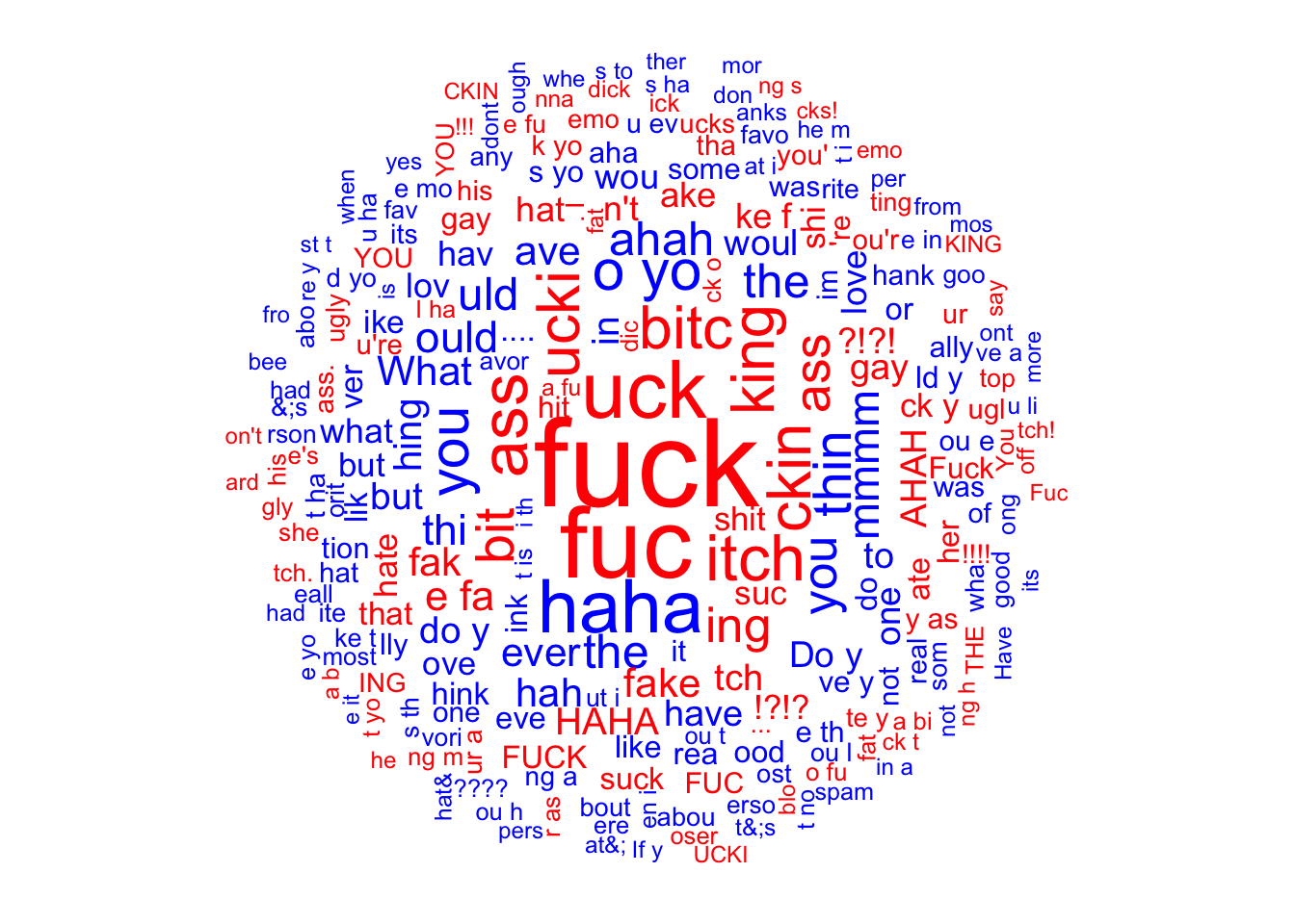
There are a number of capitalizations, long strings of repeating letters (which shingles are more likely to capture), and punctuation (e.g. ?!?!). The shingles scope of analysis seems like it is capturing some important details. This will be worthwhile if I can leverage these features in the dimensionality reduction process.

troll_ngrams <- train %>% 
  filter(label == 1) %>%
  mutate(clean_text = tm::stripWhitespace(content)) %>%
  unnest_tokens(ngram, clean_text, token = "skip_ngrams", n = 3L, k = 1) %>%
  count(ngram, sort=T) %>%
  mutate(troll_prop = n/sum(n))

notroll_ngrams <- train %>% 
  filter(label == 0) %>%
  mutate(clean_text = tm::stripWhitespace(content)) %>%
  unnest_tokens(ngram, clean_text, token = "skip_ngrams", n = 3L, k = 1) %>%
  count(ngram, sort=T) %>%
  mutate(notroll_prop = n/sum(n))

full_ngrams <- full_join(troll_ngrams, notroll_ngrams, by = "ngram") %>%
  mutate(troll_prop = ifelse(is.na(troll_prop), 0, troll_prop),
         notroll_prop = ifelse(is.na(notroll_prop), 0, notroll_prop)) %>%
  mutate(troll_notroll_diff = troll_prop - notroll_prop,
         color = ifelse(troll_notroll_diff > 0, "red", "blue"),
         abs = abs(troll_notroll_diff)) %>%
  arrange(desc(abs))

wordcloud(words = full_ngrams$ngram, freq = full_ngrams$abs, min.freq = 0,
          max.words = 150, random.order = FALSE, rot.per = 0.3, 
          colors=full_ngrams$color, ordered.colors=TRUE)

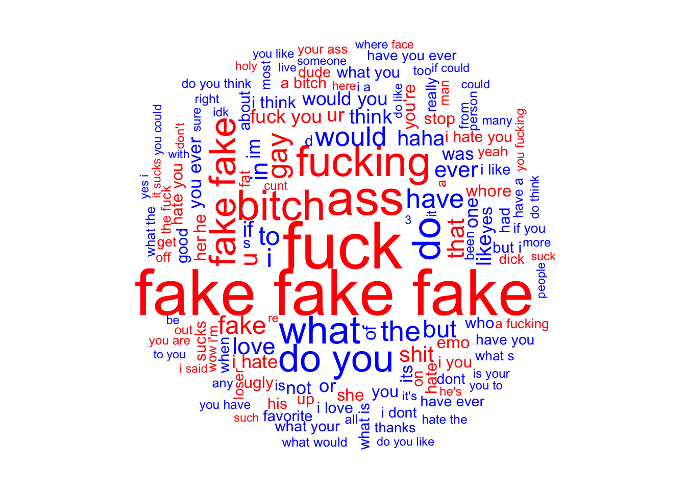
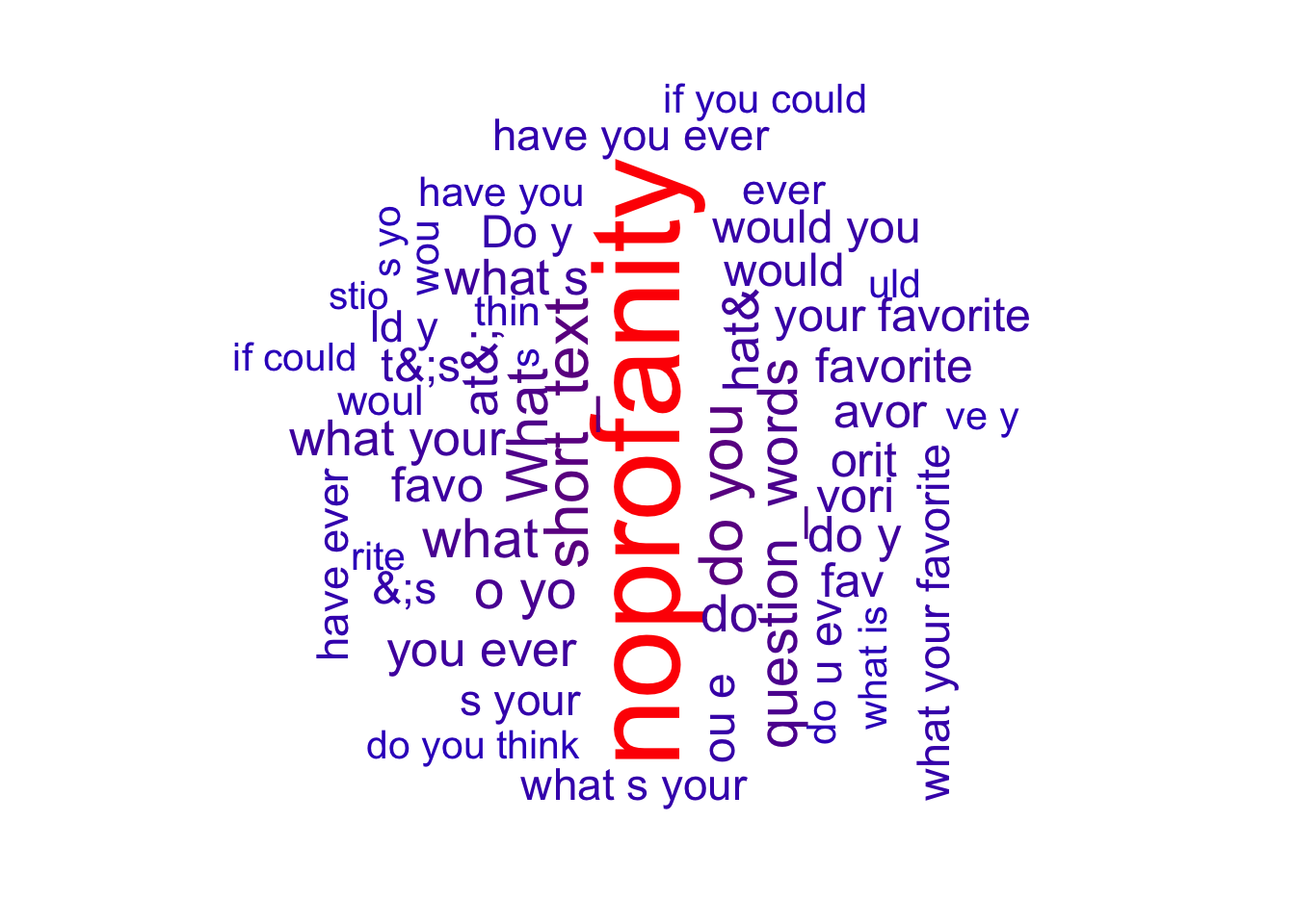
Words displaying the greatest difference in usage frequency between troll and non-troll texts.

On the level of n-grams, the most informative predictors look to be the same vulgar slurs found on the single-word level. Nevertheless, there are many multi-word sequences in this word cloud. Especially striking is the common appearance of the word “you” on both the troll and non-troll sides, in varying contexts. Whereas in single-word analysis “YOU” and “your” seemed to be indicative of trolls, n-gram level analysis makes it clear that certain phrases such as “would you”, “do you think”, “have you ever”, and “if you” are in fact much highly indicative of non-trolls. This suggests that allowing n-grams may increase the predictive abilities of the model, providing the dimentionality reduction works properly.

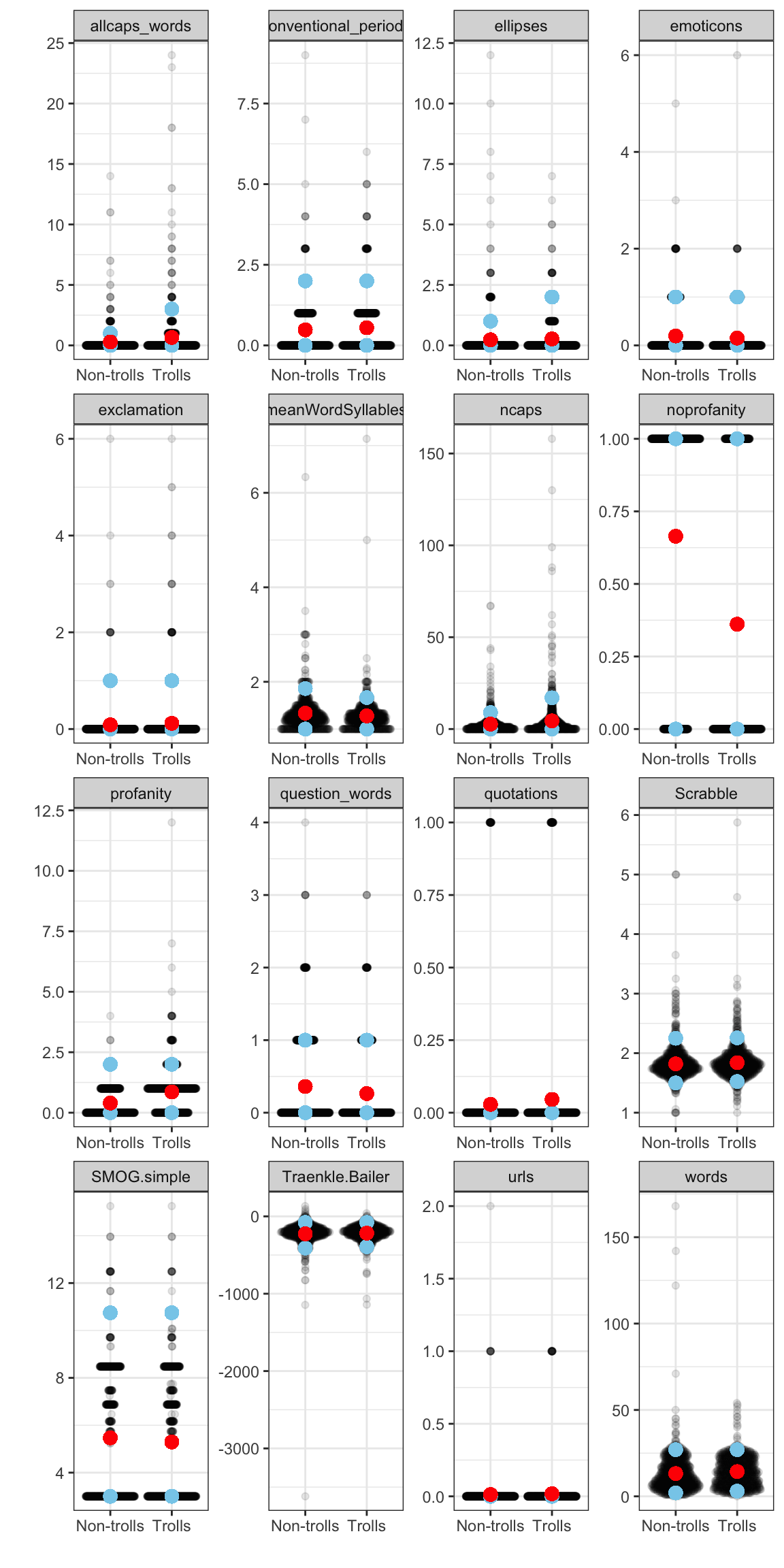
Other Important Features

While single words, shingles, and n-grams seem to cover a lot of differences between troll and non-troll texts, I can think of a few more features that may be relevant but will not be detected by any of the levels of tokenization analysis above. Here are some things that will not be captured in tokenization, but might be indicative of trolls:

• use of all-caps text
• use of punctuation in normal/unconventional ways (e.g. period at the end of sentence, three exclamation points, ***, …, quotes)
• emoticons (e.g. “:-)”, “<3”, “:3”)
• user tags
• same character many times in a row
• readability, as measured by various algorithms (e.g. “Scrabble”, “SMOG.simple”, “Traenkle.Bailer2”, “meanWordSyllables”)

# Get list of emoticons and add escapes for use as regex
emoticons <- str_replace_all(str_replace_all(lexicon::hash_emoticons$x, "\\\\", "\\\\\\\\"), "([.|()^{}+$*?]|\\[|\\])", "\\\\\\1")
count_emoticons <- function(x){
  count <- rep_len(0L, length(x))
  for (i in 1:length(emoticons)) {
    count <- count + str_count(x, emoticons[i])
  }
  count
}
question_words <- c("who", "what", "when", "where", "how", "why", "whose",
                    "Who", "What", "When", "Where", "How", "Why", "Whose",
                    "Would", "Have", "Do", "Does", "Did", "Didn't", 
                    "Didnt", "Are", "Aren't", "Arent")
count_question_words <- function(x){
  count <- rep_len(0L, length(x))
  for (i in 1:length(question_words)) {
    count <- count + str_count(x, question_words[i])
  }
  count
}
profanity <- str_replace_all(str_replace_all(lexicon::profanity_banned, "\\\\", "\\\\\\\\"), "([.|()^{}+$*?]|\\[|\\])", "\\\\\\1")
count_profanity <- function(x){
  count <- rep_len(0L, length(x))
  for (i in 1:length(profanity)) {
    count <- count + str_count(str_to_lower(x), profanity[i])
  }
  count
}

train_features <- train %>% 
  mutate(ncaps = str_count(content, "[A-Z]"), # capital Letters
         allcaps_words = str_count(content, "\\b[A-Z]{2,}\\b"), # words of ALLCAPS text
         conventional_periods = str_count(content, "[:alnum:]\\.[:space:]"), # conventionally used periods
         ellipses = str_count(content, "\\.\\."), # ...
         exclamation = str_count(content, "\\!\\!"), # !!
         emoticons = count_emoticons(content),
         question_words = count_question_words(content),
         profanity = count_profanity(content),
         noprofanity = as.integer(profanity == 0),
         urls = str_count(content, "http://"),
         words = str_count(content, '\\w+'),
         quotations = str_count(content, '".+"'))

# Readability measures
train_features <- train_features %>% 
  bind_cols(quanteda.textstats::textstat_readability(train_features$content, 
                                                     measure = c("Scrabble", 
                                                                 "SMOG.simple", 
                                                                 "Traenkle.Bailer",
                                                                 "meanWordSyllables")) %>% select(-document))

train_features %>% 
  mutate(label = if_else(label == 1, "Trolls", "Non-trolls")) %>% 
  pivot_longer(ncaps:meanWordSyllables, names_to = "feature", values_to = "value") %>% 
  group_by(label, feature) %>% 
  mutate(mean_value = mean(value, na.rm = TRUE),
         quantile_value_hi = quantile(value, probs = .95, na.rm = TRUE),
         quantile_value_lo = quantile(value, probs = .05, na.rm = TRUE)) %>% 
  slice_sample(n = 1000) %>% 
  ungroup() %>% 
  ggplot(aes(label, value)) +
    ggbeeswarm::geom_quasirandom(alpha = .1) +
    geom_point(aes(y = quantile_value_hi), color = "skyblue", size = 3) + 
    geom_point(aes(y = quantile_value_lo), color = "skyblue", size = 3) + 
    geom_point(aes(y = mean_value), color = "red", size = 3) + 
    facet_wrap(~feature, scales = "free") +
    labs(x = "", y = "") +
    theme_bw()

Some of these (e.g. conventional periods, ellipses, exclamation marks) will in fact be automatically captured by shingles. I’ll keep the ones that won’t (total emoticons, allcaps words, quotations, ncaps, question_words, profanity, lack of profanity, urls).

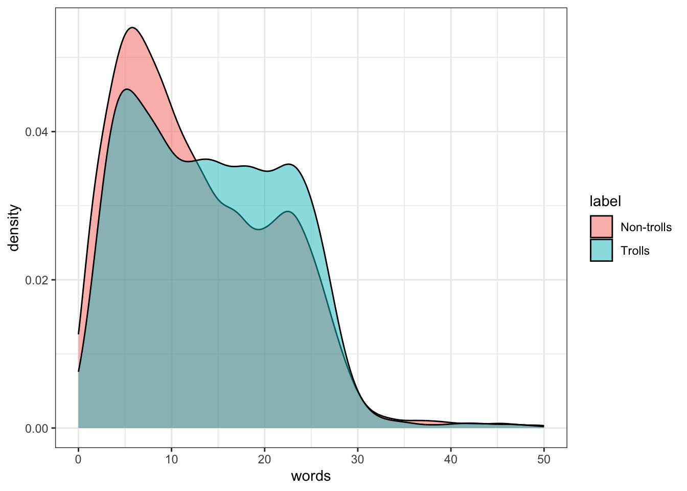
Let’s take a closer look at the number of words in each text:

train_features %>% 
  mutate(label = if_else(label == 1, "Trolls", "Non-trolls")) %>% 
  ggplot(aes(words, fill = label)) +
    geom_density(alpha = .5) +
    scale_x_continuous(limits = c(0, 50)) +
    theme_bw()

Warning: Removed 44 rows containing non-finite values (`stat_density()`).

These distributions do have notably different shapes: Non-troll texts are very commonly around 6 words long, and fall off sharply above that. Troll texts, on the other hand, are more evenly distributed between 5 and 25 words in length. This means that texts around 6 words long are disproportionately likely not to be trolls, whereas texts that are 14-26 words long are disproportionately likely to be trolls. I will therefore create two binary variables: short_text for texts under 13 words long, and med_text for texts 14-26 words long.

train_features <- train_features %>% 
  mutate(short_text = as.integer(words < 13),
         med_text = as.integer((words > 13) & (words < 27))) %>% 
  select(-words)

2. Partial Least Squares (PLS)

Partial least squares regression is a method for finding the optimal linear combinations of variables (“rotations” or “components”) for predicting an outcome, with the single hyperparameter - the number of components. This results in dramatic dimensionality reduction without discarding any variables outright, an important property for such short texts, which result in very low probability than any given n-gram or shingle will appear. PLS will treat many variables together as a unit, thereby allowing them to stand in for one another as necessary.

PLS is more fitting for this task than principle components regression (PCR), a similar technique which calculates the components based on variance explained in the predictors rather than in the outcome. This is because trolls write in varying conversational contexts, so the directions of maximal variance in the predictors are likely to reflect these trivial topical differences rather than the differences between trolls and non-trolls. PLS solves this problem by directly optimizing the rotations for prediction of troll status.

Since this model is designed for a Kaggle competition with a hidden test set, I will split the training set here into a further train and test set for the purpose of evaluating models during production. When the best model is established, I will retrain it on the full set.

# find 1000 shingles with the greatest absolute difference between groups, scaled by overall frequency
top_shingles <- full_shingles %>% 
  arrange(desc(abs*(troll_prop + notroll_prop))) %>% 
  slice_head(n = 1000) %>% 
  pull(shingle)

# add shingles to other features as sparse features
train_allfeatures <- train_features %>% 
  select(c(rowid, content, label, allcaps_words, emoticons, question_words, profanity, noprofanity, quotations, SMOG.simple, Traenkle.Bailer, short_text, med_text)) %>%
  mutate(label = factor(label),
         clean_text = tm::stripWhitespace(content)) %>%
  ## Compute shingles
  unnest_tokens(shingle, clean_text, token = "character_shingles", n = 4L,
                strip_non_alphanum = FALSE, to_lower = FALSE, drop = FALSE) %>% 
  # replace everything but top 1000 with placeholder
  mutate(shingle = if_else(shingle %in% top_shingles, shingle, "shingle")) %>% 
  group_by(across(everything())) %>% summarise(n = n()) %>% ungroup() %>% 
  # pivot shingles to columns
  pivot_wider(id_cols = rowid:clean_text, names_from = "shingle", values_from = "n", names_prefix = "shingle_", values_fill = 0L) %>% 
  mutate(across(everything(), ~replace_na(.x, 0))) %>% 
  ungroup()

# Split test into test and train
set.seed(123)
training_samples <- train_allfeatures$label %>% createDataPartition(p = 0.8, list = FALSE)
train_allfeatures.train  <- train_allfeatures[training_samples, ]
train_allfeatures.test <- train_allfeatures[-training_samples, ]

# PLS Model (10-fold cross-validation)
set.seed(123)
pls_mod <- train(
  label~., data = select(train_allfeatures.train, -c(rowid, content, clean_text)), method = "pls",
  scale = TRUE,
  trControl = trainControl("cv", number = 10),
  tuneLength = 20
  )

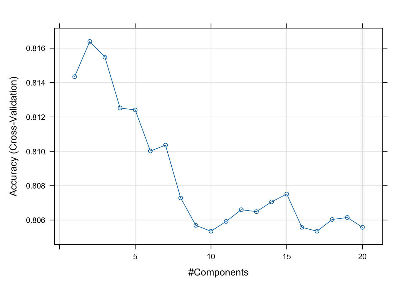
# Plot model CV accuracy vs different values of components
plot(pls_mod) # 2 components in optimal

Cross-validation indicated that 2 components is optimal. Each of these components represents a weighted ensemble of variables that tend to hang together in the way they relate to troll status.

# EVALUATE
pls_pred <- predict(pls_mod,
                    ncomp = pls_mod$bestTune$ncomp,
                    newdata = train_allfeatures.test) 
RMSE(as.integer(pls_pred), as.integer(train_allfeatures.test$label))
# Test RMSE = 0.4236731
pls_confmat <- confusionMatrix(pls_pred, train_allfeatures.test$label)
# Test accuracy: 0.8205
# Sensitivity : 0.9798          
# Specificity : 0.1373

82% test accuracy is respectable. Let’s try again, this time including the 1000 top n-grams on top of the shingles.

# find 1500 ngrams with the greatest absolute difference between groups, scaled by overall frequency
top_ngrams <- full_ngrams %>% 
  arrange(desc(abs*(troll_prop + notroll_prop))) %>% 
  slice_head(n = 1000) %>% 
  pull(ngram)

# add ngrams to other features as sparse features
train_allfeatures_ngrams <- train_features %>% 
  select(c(rowid, content)) %>%
  mutate(clean_text = tm::stripWhitespace(content)) %>%
  ## Compute ngrams
  unnest_tokens(ngram, clean_text, token = "skip_ngrams", n = 3L, k = 1) %>%
  # replace everything but top 1000 with placeholder
  mutate(ngram = if_else(ngram %in% top_ngrams, ngram, "ngram")) %>% 
  group_by(across(everything())) %>% summarise(n = n()) %>% ungroup() %>% 
  # pivot ngrams to columns
  pivot_wider(id_cols = rowid:content, names_from = "ngram", values_from = "n", names_prefix = "ngram_", values_fill = 0L) %>% 
  mutate(across(everything(), ~replace_na(.x, 0))) %>% 
  full_join(train_allfeatures %>% select(-c(clean_text)))

# resplit test into test and train (same split as before)
train_allfeatures_ngrams.train  <- train_allfeatures_ngrams[training_samples, ]
train_allfeatures_ngrams.test <- train_allfeatures_ngrams[-training_samples, ]

# PLS Model (10-fold cross-validation)
set.seed(123)
pls_ngram_mod <- train(
  label~., data = select(train_allfeatures_ngrams.train, -c(rowid, content), -any_of(nzv)), method = "pls",
  scale = TRUE,
  trControl = trainControl("cv", number = 10),
  tuneLength = 20
  )

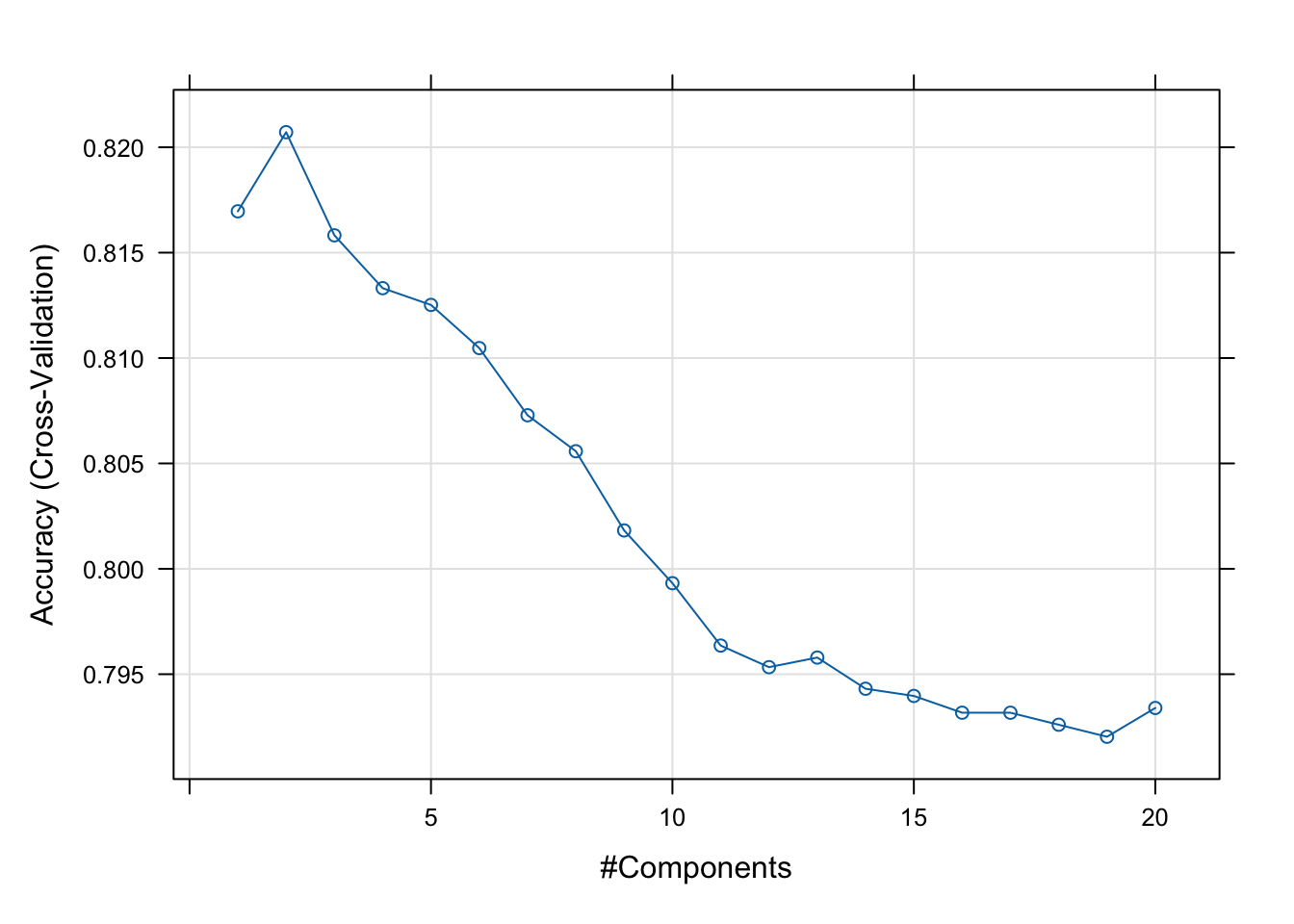
# Plot model RMSE vs different values of components
plot(pls_ngram_mod)

Again 2 components is optimal, according to the CV metrics.

pls_ngram_mod$bestTune

# EVALUATE
pls_ngram_pred <- predict(pls_ngram_mod,
                          ncomp = pls_ngram_mod$bestTune$ncomp,
                          newdata = train_allfeatures_ngrams.test)
RMSE(as.integer(pls_ngram_pred), as.integer(train_allfeatures_ngrams.test$label))
# Test RMSE = 0.4166249
pls_ngram_confmat <- confusionMatrix(pls_ngram_pred, train_allfeatures_ngrams.test$label)
# Test accuracy: 0.8251  Slightly better than the last one
# Sensitivity : 0.9770   Sensitivity is lower  
# Specificity : 0.1735   Specificity is higher

Test accuracy is only very slightly better with n-grams than without. Does this mean the model is not using the n-grams at all? To answer this question, I’ll take a peek at the top variable loadings of the components being used here.

pls_ngram_loadings <- loadings(pls_ngram_mod$finalModel)

# PC1-PC3 Top Loadings:
head(as.data.frame(pls_ngram_loadings[,1:2]))

                       Comp 1        Comp 2
ngram_a          -0.037442868  0.0805943518
ngram_gay        -0.020795963 -0.0472275494
ngram_girls       0.006310189 -0.0002616247
ngram_going      -0.021373361  0.0681882011
`ngram_going to` -0.021525804  0.0623300444
ngram_how         0.006202302 -0.0109130778

wordcloud(words = str_remove_all(str_remove(names(pls_ngram_loadings[,1]), "shingle_|ngram_"), "`"), 
          freq = pls_ngram_loadings[,1], min.freq = 0, colors = colorRampPalette(c("blue", "red"))(2000),
          max.words = 50, random.order = FALSE, rot.per = 0.2)

wordcloud(words = str_remove_all(str_remove(names(pls_ngram_loadings[,2]), "shingle_|ngram_"), "`"), 
          freq = pls_ngram_loadings[,2], min.freq = 0,
          colors = colorRampPalette(c("blue", "red"))(2000),
          max.words = 50, random.order = FALSE, rot.per = 0.2)

The first component, it seems, is dominated by the binary appearance of profanity or lack thereof, with most of the rest of the weight given to question words. Interestingly, the second component is dominated by the placeholder variables “shingle” and “ngram”, representing the count of tokens not counted individually (i.e. not in the list of 1000 most informative ngrams/shingles).

3. Boosting

The revelation that the PLS components are dominated by my custom-made features is somewhat concerning. Aside from those custom-made features, the PLS model had access to thousands of shingles and n-grams. While this allows the model to pick up on more detail, it opens the door to the pernicious influence of random noise. PLS is designed to counteract this by combining the variables into components rather than treating them individually, but it is nevertheless worthwhile to be wary of the “let’s throw in as many variables as possible” approach to machine learning.

To see whether including all those thousands of tokens was worth the variance it may have introduced, I’ll train another model on only the custom-made features explored above. For this model, I’m using boosting, a method of aggregating many weak models, each optimized to explain the variance left over by those before it. The aggregation of many models has the effect of regularization - minimizing the effect of noisy variables - in a similar way to PLS.

# resplit test into test and train (same split as before)
train_features.train  <- train_features[training_samples, ]
train_features.test <- train_features[-training_samples, ]

tg <- expand.grid(interaction.depth = c(1, 2, 3),  # tree-depth: catch interactions (d)
                  n.trees = 10000,  # 10000 trees (B)
                  shrinkage = 0.005, # slow learning rate
                  n.minobsinnode = 10 # minimum 10 observations per node of tree
                  )

# Boosting Model (10-fold cross-validation)
set.seed(123)
boost_customfeatures_mod <- train(
  label~., data = select(train_features.train, -c(rowid, content)), method = "gbm",
  tuneGrid = tg,
  na.action  = na.pass,
  trControl = trainControl("cv", number = 10)
  )
# Plot model accuracy vs different values of components
plot(boost_ngram_mod) # Tree-depth = 1 ("stumps") are best, a common finding
summary(boost_ngram_mod)

# EVALUATE
boost_customfeatures_pred <- predict(boost_customfeatures_mod, 
                                     interaction.depth = 1,
                                     newdata = train_features.test) 

boost_customfeatures_confmat <- confusionMatrix(boost_customfeatures_pred, na.omit(train_features.test)$label)
# Test accuracy: 0.8089  Not as good as full PLS
# Sensitivity : 0.98533   Sensitivity is higher   
# Specificity : 0.05542   Specificity is lower

The performance of this model is respectable, but not as good as the full PLS model. Specifically, the sensitivity (for identifying non-trolls) is much higher, and the specificity much lower. This indicates that the model is leveraging the unbalanced dataset by guessing that most texts are not trolls.

Retrain best model on full training set

Now that the PLS model incorporating n-grams and shingles is established as the superior one, I will retrain it on the full training dataset before submitting it to the Kaggle competition.

# Full-set PLS Model (10-fold cross-validation)
# Using feature set with ngrams
set.seed(123)
pls_mod_final <- train(
  label~., data = select(train_allfeatures, -c(rowid, content, clean_text)), method = "pls",
  scale = TRUE,
  trControl = trainControl("cv", number = 10),
  tuneLength = 4
  )

plot(pls_mod_final) # Still best with 2 components

# Identify features found in train but not test set
test <- read_csv("test.csv")

test_shingles <- test %>% 
  mutate(clean_text = tm::stripWhitespace(content)) %>%
  unnest_tokens(shingle, clean_text, token = "character_shingles", n = 4L,
                strip_non_alphanum = FALSE, to_lower = FALSE) %>%
  count(shingle, sort=T)
irrelevant_shingles <- setdiff(top_shingles, test_shingles$shingle) # none missing!

test_ngrams <- test %>% 
  mutate(clean_text = tm::stripWhitespace(content)) %>%
  unnest_tokens(ngram, clean_text, token = "skip_ngrams", n = 3L, k = 1) %>%
  count(ngram, sort=T)
irrelevant_ngrams <- setdiff(top_ngrams, test_ngrams$ngram) # list of 7

# Add all features to test set

test_features <- test %>% 
  mutate(ncaps = str_count(content, "[A-Z]"), # capital Letters
         allcaps_words = str_count(content, "\\b[A-Z]{2,}\\b"), # words of ALLCAPS text
         conventional_periods = str_count(content, "[:alnum:]\\.[:space:]"), # conventionally used periods
         ellipses = str_count(content, "\\.\\."), # ...
         exclamation = str_count(content, "\\!\\!"), # !!
         emoticons = count_emoticons(content),
         question_words = count_question_words(content),
         profanity = count_profanity(content),
         noprofanity = as.integer(profanity == 0),
         urls = str_count(content, "http://"),
         words = str_count(content, '\\w+'),
         quotations = str_count(content, '".+"'),
         short_text = as.integer(words < 13),
         med_text = as.integer((words > 13) & (words < 27)),
         clean_text = tm::stripWhitespace(content)) %>% 
  # Readability measures and quantized length
  bind_cols(quanteda.textstats::textstat_readability(test_features$content, 
                                                     measure = c("Scrabble", 
                                                                 "SMOG.simple", 
                                                                 "Traenkle.Bailer",
                                                                 "meanWordSyllables"))) %>% 
  select(c(rowid, content, allcaps_words, emoticons, question_words, profanity, noprofanity, quotations, SMOG.simple, Traenkle.Bailer, short_text, med_text, clean_text)) %>%
  ## Compute shingles
  unnest_tokens(shingle, clean_text, token = "character_shingles", n = 4L,
                strip_non_alphanum = FALSE, to_lower = FALSE, drop = FALSE) %>% 
  # replace everything but top 1000 with placeholder
  mutate(shingle = if_else(shingle %in% top_shingles, shingle, "shingle")) %>% 
  group_by(across(everything())) %>% summarise(n = n()) %>% ungroup() %>% 
  # pivot shingles to columns
  pivot_wider(id_cols = rowid:clean_text, names_from = "shingle", values_from = "n", names_prefix = "shingle_", values_fill = 0L) %>% 
  mutate(across(everything(), ~replace_na(.x, 0))) %>% 
  ungroup()

# add ngrams to other features as sparse features
test_features <- test_features %>% 
  select(c(rowid, content)) %>%
  mutate(clean_text = tm::stripWhitespace(content)) %>%
  ## Compute ngrams
  unnest_tokens(ngram, clean_text, token = "skip_ngrams", n = 3L, k = 1) %>%
  # replace everything but top 1000 with placeholder
  mutate(ngram = if_else(ngram %in% top_ngrams, ngram, "ngram")) %>% 
  group_by(across(everything())) %>% summarise(n = n()) %>% ungroup() %>% 
  # pivot ngrams to columns
  pivot_wider(id_cols = rowid:content, names_from = "ngram", values_from = "n", names_prefix = "ngram_", values_fill = 0L) %>% 
  mutate(across(everything(), ~replace_na(.x, 0))) %>% 
  full_join(test_features %>% select(-c(clean_text)))

# Add train-unique features in with all zeros
paste0("ngram_", irrelevant_ngrams)
test_features <- test_features %>% 
  mutate(`ngram_fake fake fake` = 0, `ngram_fake fake` = 0,
         `ngram_whore whore` = 0, `ngram_it fuck` = 0,
         `ngram_fuck u` = 0, `ngram_a a a` = 0,
         `ngram_lick` = 0)

# Predictions to csv
data.frame(Id = test_features$rowid,
           Category = predict(pls_mod_final,
                              ncomp = pls_mod_final$bestTune$ncomp,
                              newdata = test_features)) %>%  
  write_csv("~/Downloads/pls_mod_predictions.csv")

4. Tuned Transformer

The workflow outlined above, with exploratory data analysis and feature selection, is a hallmark of traditional machine learning. Nowadays, however, the cutting edge of the field is dominated by a much more hands-off approach, powered by deep neural networks. In recent years, this approach has become more accessible than ever with the rise of transfer learning - On platforms like Hugging Face, large pre-trained language models are freely available to fine-tune on specialized datasets. Fine-tuning is computationally inexpensive and is possible to do in a matter of hours on a personal computer or in the cloud with Google Colab. Given the accessibility of such cutting-edge methods, I decided to train a deep learning model on the troll data. If tuned correctly, this will give a reasonable upper bound on the maximum accuracy one could hope to achieve on these data. After all, the texts in the dataset are short, and the lack of contextual information may make it difficult even for humans to distinguish trolls from non-trolls.

Using the Hugging Face transformers library in Python, I fine-tuned the distilbert-base-cased model on the data, and performed a hyperparameter search using the optuna library to determine the optimal learning rate, batch size, and weight decay. In light of the importance of capitalization observed in the exploratory analysis here, I used a cased model. The full Python code can be found here. I dubbed the fine-tuned distillbert “distrollbert”. It is available on the Hugging Face hub.

Suffice it to say, the distrollbert performed better than any of the models explored above, but not dramatically so.